PyData NYC ‘23#

E-graphs in Python with egglog

Saul Shanabrook

Aims:#

Faithful bindings for egglog rust library.
“Pythonic” interface, using standard type definitions.
Usable as base for optimizing/translating expressions for data science libraries in Python

What is an e-graph?#

E-graphs are these super wonderful data structures for managing equality and equivalence information. They are traditionally used inside of constraint solvers and automated theorem provers to implement congruence closure, an efficient algorithm for equational reasoning—but they can also be used to implement rewrite systems.

Talia Ringer - “Proof Automation” course

Define types and functions/operators
Define rewrite rules
Add expressions to graph
Run rewrite rules on expressions until saturated (addtional applications have no effect)
Extract out lowest cost expression

Example#

from __future__ import annotations
from egglog import *

egraph = EGraph()


@egraph.class_
class NDArray(Expr):
    def __init__(self, i: i64Like) -> None:
        ...

    def __add__(self, other: NDArray) -> NDArray:
        ...

    def __mul__(self, other: NDArray) -> NDArray:
        ...


@egraph.function(cost=2)
def arange(i: i64Like) -> NDArray:
    ...


# Register rewrite rule that asserts for all values x of type NDArray
# x + x = x * 2
x = var("x", NDArray)
egraph.register(rewrite(x + x).to(x * NDArray(2)))

res = arange(10) + arange(10)
egraph.register(res)
egraph.saturate()

egraph.extract(res)

arange(10) * NDArray(2)

Example with Scikit-learn#

Optimize Scikit-learn function with Numba by building an e-graph that implements the Array API.

from sklearn import config_context
from sklearn.datasets import make_classification
from sklearn.discriminant_analysis import LinearDiscriminantAnalysis


def run_lda(x, y):
    with config_context(array_api_dispatch=True):
        lda = LinearDiscriminantAnalysis()
        return lda.fit(x, y).transform(x)


X_np, y_np = make_classification(random_state=0, n_samples=1000000)
run_lda(X_np, y_np)

array([[ 0.64233002],
       [ 0.63661245],
       [-1.603293  ],
       ...,
       [-1.1506433 ],
       [ 0.71687176],
       [-1.51119579]])

from egglog.exp.array_api import *
from egglog.exp.array_api_jit import jit


@jit
def optimized_fn(X, y):
    # Add metadata about input shapes and dtypes, so that abstract array
    # can pass scikit-learn runtime checks
    assume_dtype(X, X_np.dtype)
    assume_shape(X, X_np.shape)
    assume_isfinite(X)

    assume_dtype(y, y_np.dtype)
    assume_shape(y, y_np.shape)
    assume_value_one_of(y, (0, 1))

    return run_lda(X, y)

Here is an example of a rewrite rule we used to generate Numba compatible code:

rewrite(
    std(x, axis)
).to(
    sqrt(mean(square(x - mean(x, axis, keepdims=TRUE)), axis))
)

We can see the optimized expr:

optimized_fn.expr

_NDArray_1 = NDArray.var("X")
assume_dtype(_NDArray_1, DType.float64)
assume_shape(_NDArray_1, TupleInt(Int(1000000)) + TupleInt(Int(20)))
assume_isfinite(_NDArray_1)
_NDArray_2 = NDArray.var("y")
assume_dtype(_NDArray_2, DType.int64)
assume_shape(_NDArray_2, TupleInt(Int(1000000)))
assume_value_one_of(_NDArray_2, TupleValue(Value.int(Int(0))) + TupleValue(Value.int(Int(1))))
_NDArray_3 = astype(
    NDArray.vector(TupleValue(sum(_NDArray_2 == NDArray.scalar(Value.int(Int(0)))).to_value()) + TupleValue(sum(_NDArray_2 == NDArray.scalar(Value.int(Int(1)))).to_value())),
    DType.float64,
) / NDArray.scalar(Value.float(Float(1000000.0)))
_NDArray_4 = zeros(TupleInt(Int(2)) + TupleInt(Int(20)), OptionalDType.some(DType.float64), OptionalDevice.some(_NDArray_1.device))
_MultiAxisIndexKey_1 = MultiAxisIndexKey(MultiAxisIndexKeyItem.slice(Slice()))
_IndexKey_1 = IndexKey.multi_axis(MultiAxisIndexKey(MultiAxisIndexKeyItem.int(Int(0))) + _MultiAxisIndexKey_1)
_NDArray_5 = _NDArray_1[ndarray_index(_NDArray_2 == NDArray.scalar(Value.int(Int(0))))]
_OptionalIntOrTuple_1 = OptionalIntOrTuple.some(IntOrTuple.int(Int(0)))
_NDArray_4[_IndexKey_1] = sum(_NDArray_5, _OptionalIntOrTuple_1) / NDArray.scalar(Value.int(_NDArray_5.shape[Int(0)]))
_IndexKey_2 = IndexKey.multi_axis(MultiAxisIndexKey(MultiAxisIndexKeyItem.int(Int(1))) + _MultiAxisIndexKey_1)
_NDArray_6 = _NDArray_1[ndarray_index(_NDArray_2 == NDArray.scalar(Value.int(Int(1))))]
_NDArray_4[_IndexKey_2] = sum(_NDArray_6, _OptionalIntOrTuple_1) / NDArray.scalar(Value.int(_NDArray_6.shape[Int(0)]))
_NDArray_7 = concat(TupleNDArray(_NDArray_5 - _NDArray_4[_IndexKey_1]) + TupleNDArray(_NDArray_6 - _NDArray_4[_IndexKey_2]), OptionalInt.some(Int(0)))
_NDArray_8 = square(_NDArray_7 - expand_dims(sum(_NDArray_7, _OptionalIntOrTuple_1) / NDArray.scalar(Value.int(_NDArray_7.shape[Int(0)]))))
_NDArray_9 = sqrt(sum(_NDArray_8, _OptionalIntOrTuple_1) / NDArray.scalar(Value.int(_NDArray_8.shape[Int(0)])))
_NDArray_10 = copy(_NDArray_9)
_NDArray_10[ndarray_index(_NDArray_9 == NDArray.scalar(Value.int(Int(0))))] = NDArray.scalar(Value.float(Float(1.0)))
_TupleNDArray_1 = svd(sqrt(NDArray.scalar(Value.float(Float.rational(Rational(1, 999998))))) * (_NDArray_7 / _NDArray_10), FALSE)
_Slice_1 = Slice(OptionalInt.none, OptionalInt.some(sum(astype(_TupleNDArray_1[Int(1)] > NDArray.scalar(Value.float(Float(0.0001))), DType.int32)).to_value().to_int))
_NDArray_11 = (_TupleNDArray_1[Int(2)][IndexKey.multi_axis(MultiAxisIndexKey(MultiAxisIndexKeyItem.slice(_Slice_1)) + _MultiAxisIndexKey_1)] / _NDArray_10).T / _TupleNDArray_1[
    Int(1)
][IndexKey.slice(_Slice_1)]
_TupleNDArray_2 = svd(
    (sqrt((NDArray.scalar(Value.int(Int(1000000))) * _NDArray_3) * NDArray.scalar(Value.float(Float(1.0)))) * (_NDArray_4 - (_NDArray_3 @ _NDArray_4)).T).T @ _NDArray_11, FALSE
)
(
    (_NDArray_1 - (_NDArray_3 @ _NDArray_4))
    @ (
        _NDArray_11
        @ _TupleNDArray_2[Int(2)].T[
            IndexKey.multi_axis(
                _MultiAxisIndexKey_1
                + MultiAxisIndexKey(
                    MultiAxisIndexKeyItem.slice(
                        Slice(
                            OptionalInt.none,
                            OptionalInt.some(
                                sum(astype(_TupleNDArray_2[Int(1)] > (NDArray.scalar(Value.float(Float(0.0001))) * _TupleNDArray_2[Int(1)][IndexKey.int(Int(0))]), DType.int32))
                                .to_value()
                                .to_int
                            ),
                        )
                    )
                )
            )
        ]
    )
)[IndexKey.multi_axis(_MultiAxisIndexKey_1 + MultiAxisIndexKey(MultiAxisIndexKeyItem.slice(Slice(OptionalInt.none, OptionalInt.some(Int(1))))))]

And the generated code:

import inspect

print(inspect.getsource(optimized_fn))

def __fn(X, y):
    assert X.dtype == np.dtype(np.float64)
    assert X.shape == (1000000, 20,)
    assert np.all(np.isfinite(X))
    assert y.dtype == np.dtype(np.int64)
    assert y.shape == (1000000,)
    assert set(np.unique(y)) == set((0, 1,))
    _0 = y == np.array(0)
    _1 = np.sum(_0)
    _2 = y == np.array(1)
    _3 = np.sum(_2)
    _4 = np.array((_1, _3,)).astype(np.dtype(np.float64))
    _5 = _4 / np.array(1000000.0)
    _6 = np.zeros((2, 20,), dtype=np.dtype(np.float64))
    _7 = np.sum(X[_0], axis=0)
    _8 = _7 / np.array(X[_0].shape[0])
    _6[0, :] = _8
    _9 = np.sum(X[_2], axis=0)
    _10 = _9 / np.array(X[_2].shape[0])
    _6[1, :] = _10
    _11 = _5 @ _6
    _12 = X - _11
    _13 = np.sqrt(np.array(float(1 / 999998)))
    _14 = X[_0] - _6[0, :]
    _15 = X[_2] - _6[1, :]
    _16 = np.concatenate((_14, _15,), axis=0)
    _17 = np.sum(_16, axis=0)
    _18 = _17 / np.array(_16.shape[0])
    _19 = np.expand_dims(_18, 0)
    _20 = _16 - _19
    _21 = np.square(_20)
    _22 = np.sum(_21, axis=0)
    _23 = _22 / np.array(_21.shape[0])
    _24 = np.sqrt(_23)
    _25 = _24 == np.array(0)
    _24[_25] = np.array(1.0)
    _26 = _16 / _24
    _27 = _13 * _26
    _28 = np.linalg.svd(_27, full_matrices=False)
    _29 = _28[1] > np.array(0.0001)
    _30 = _29.astype(np.dtype(np.int32))
    _31 = np.sum(_30)
    _32 = _28[2][:_31, :] / _24
    _33 = _32.T / _28[1][:_31]
    _34 = np.array(1000000) * _5
    _35 = _34 * np.array(1.0)
    _36 = np.sqrt(_35)
    _37 = _6 - _11
    _38 = _36 * _37.T
    _39 = _38.T @ _33
    _40 = np.linalg.svd(_39, full_matrices=False)
    _41 = np.array(0.0001) * _40[1][0]
    _42 = _40[1] > _41
    _43 = _42.astype(np.dtype(np.int32))
    _44 = np.sum(_43)
    _45 = _33 @ _40[2].T[:, :_44]
    _46 = _12 @ _45
    return _46[:, :1]

As well as the e-graph:

optimized_fn.egraph

../_images/f6d8d0a9f14791da1f9f77248ae1a3d8f1cf838cf5c6c54275143f61c81db98d.svg

import numba
import numpy as np

numba_fn = numba.njit(fastmath=True)(optimized_fn)
assert np.allclose(run_lda(X_np, y_np), numba_fn(X_np, y_np))

/var/folders/xn/05ktz3056kqd9n8frgd6236h0000gn/T/egglog-82012193-cafe-439c-94d4-48ec846ca9e6.py:56: NumbaPerformanceWarning: '@' is faster on contiguous arrays, called on (Array(float64, 2, 'C', False, aligned=True), Array(float64, 2, 'A', False, aligned=True))
  _45 = _33 @ _40[2].T[:, :_44]

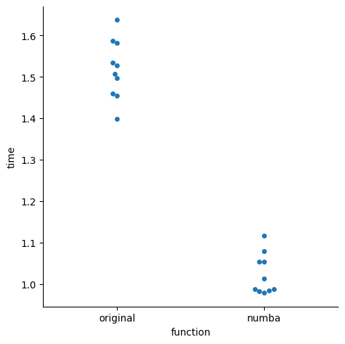
~30% speedup#

on my machine, not a scientific benchmark

import seaborn as sns

df_melt = pd.melt(df, var_name="function", value_name="time")
_ = sns.catplot(data=df_melt, x="function", y="time", kind="swarm")

../_images/6b076a0e2fcb53ded25de278f3db480efbbb19f2d9d67b3f1dc3302c4554a1bb.png

Conclusions#

egglog is a Python interface to e-graphs, which respects the underlying semantics but provides a Python interface.
Flexible enough to represent Array API and translate this back to Python source
If you have a Python library which optimizes/translates expressions, try it out!
Goals
- support the ecosystem in collaborating better between libraries, to encourage experimentation and innovation
- dont reimplement the world: build on academic programming language research
pip install egglog
https://github.com/egraphs-good/egglog-python
Say hello: https://egraphs.zulipchat.com/

Optimizing Scikit-Learn with Array API and Numba egglog

2023-11-04

Recent Posts